

The question
A retail bank’s direct-marketing team sells term deposits by phone. About 11% of past contacts subscribed, so most calls are wasted. The team wants to call the most promising clients first. The project folder held three things: the data, its data dictionary, and a short README.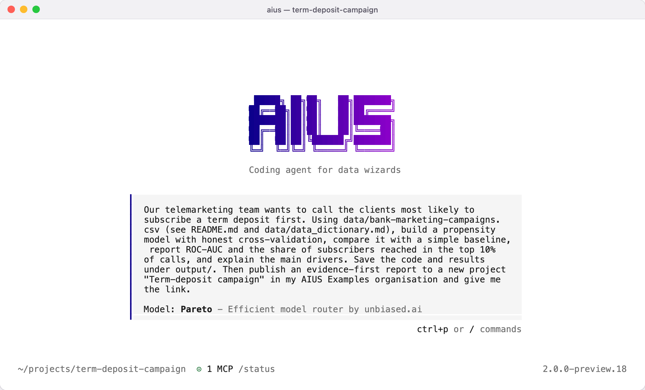
What the agent did
Read the brief and checked the environment
It read
README.md and the data dictionary, confirmed the project’s
.venv had scikit-learn, pandas and DuckDB, looked up the dataset’s source
page and created the project in AIUS Examples.Profiled the data before modelling
It found 41,188 rows, no missing values, 12 duplicate rows and 11.27% of
contacts subscribing. It flagged 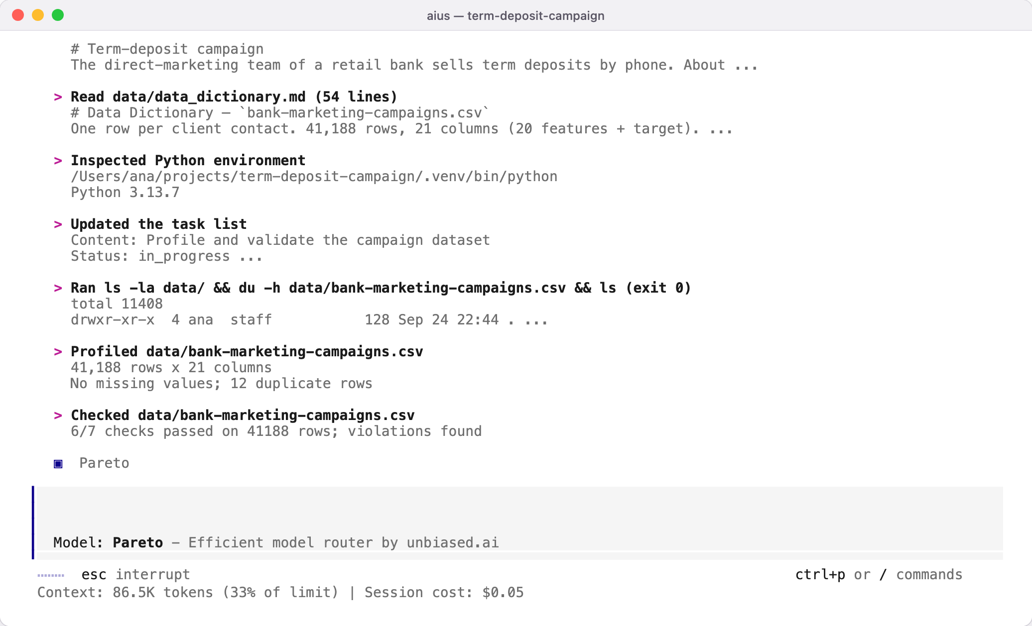
duration (the length of the last call) as
leakage: it is only known after the call it is meant to predict. It also
treated pdays = 999 as “never contacted before”, not as a number of days.Noticed that time matters
The rows are in the order the calls were made, and subscription rose from
2.8% of contacts in the first tenth to 45.9% in the last. A random
train/test split would mix past and future and overstate performance, so the
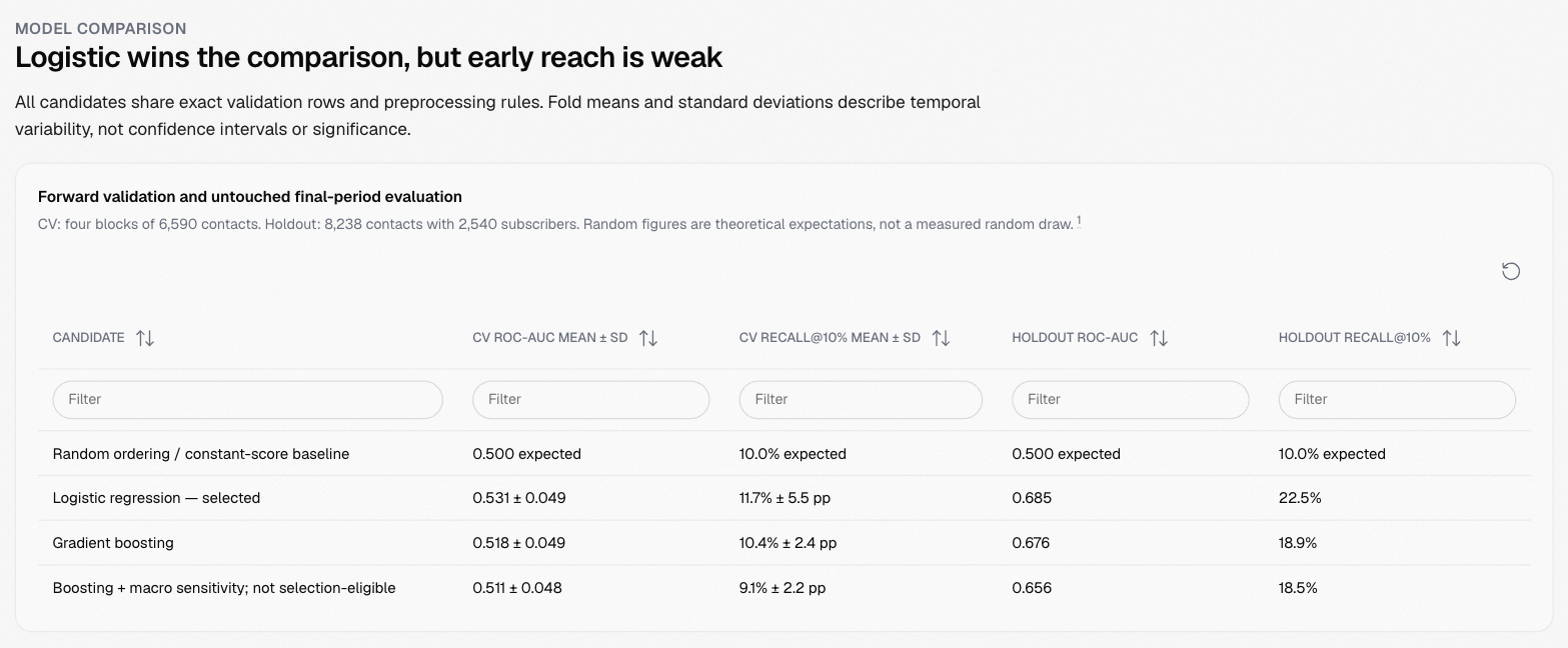
agent used forward validation: four folds of 6,590 contacts, each
trained only on earlier rows, then one untouched final period of 8,238
contacts.
Kept only what is known before a call
The model uses the client profile and previous-campaign history. It leaves
out the call’s duration, the current campaign’s contact count, the channel
and calendar fields, which are not known when the call list is drawn up.
Economic indicators were tested separately as a sensitivity check.
Compared against baselines and checked its own numbers
It compared logistic regression with gradient boosting and a random
ordering, then wrote a separate verifier. The verifier recalculated all 15
ROC-AUC and top-decile results independently and reproduced the full run
from scratch with identical results.
The result
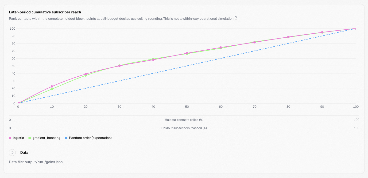
Forward CV is the mean ROC-AUC, ± its standard deviation, over the four forward folds. Final period is the ROC-AUC on the untouched last 8,238 contacts. Top 10% reach is the share of that period’s subscribers found among its top-scored 10% of contacts.| Model | Forward CV | Final period | Top 10% reach |
|---|---|---|---|
| Random ordering | 0.500 | 0.500 | 10.0% |
| Logistic regression (selected) | 0.531 ± 0.049 | 0.685 | 22.5% (571 of 2,540) |
| Gradient boosting | 0.518 ± 0.049 | 0.676 | 18.9% |
Published scores for this dataset vary a lot with the validation design and
the features allowed. This analysis kept to data known before a call and
validated forward in time, so its scores are lower and more cautious; the
report explains why.
The published report
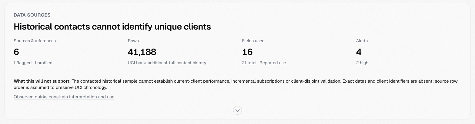
The report leads with the decision and its uncertainty, then shows the data’s limits, the model comparison, the drivers and the method. Its numbers carry footnotes to the attached files they came from.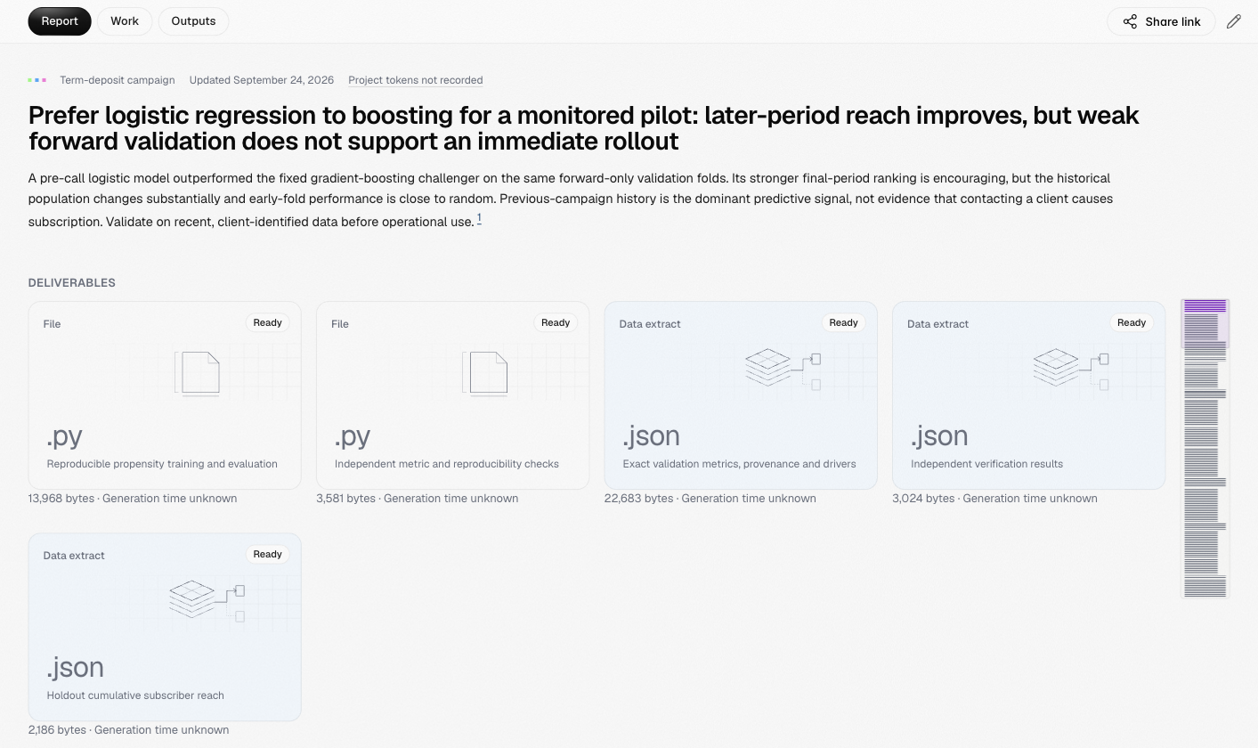
Try it yourself
Download the dataset from the UCI page above, put it indata/ with a short
README, create a .venv as in Installation, and give
the agent the same prompt with your own organisation’s name. Expect different
wording; the agent works through the same checks.